what is the ratio of mean velocity to maximum velocity?
Next: Effusion Up: Applications of Statistical Thermodynamics Previous: Specific Heats of Solids
Maxwell Velocity Distribution
Consider a molecule of mass 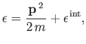 | (seven.202) |
where
 | (7.203) |
where
 | (seven.204) |
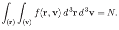
Of course, we tin can multiply this probability by the total number of molecules,
Suppose that we at present wish to determine ![]() : that is, the mean number of molecules with positions between
: that is, the mean number of molecules with positions between ![]() and
and ![]() , and velocities in the range
, and velocities in the range ![]() and
and ![]() . Considering
. Considering ![]() , it is easily seen that
, it is easily seen that
 | (7.205) |
where
 | (7.206) |
In other give-and-take, the sum over molecules with all possible positions and velocities gives the full number of molecules,
![$\displaystyle C V \left[\int_{-\infty}^{\infty} \exp\left(-\frac{\beta m v_z^{ 2}}{2}\right) dv_z\right]^{ 3} = N.$](https://farside.ph.utexas.edu/teaching/sm1/Thermalhtml/img1698.png) | (7.207) |
Now,
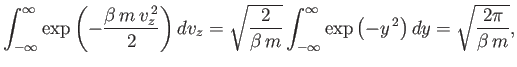 | (vii.208) |
and so
 | (7.209) |
Here,
Let united states consider the distribution of a given component of velocity: the ![]() -component (say). Suppose that
-component (say). Suppose that ![]() is the average number of molecules per unit volume with the
is the average number of molecules per unit volume with the ![]() -component of velocity in the range
-component of velocity in the range ![]() to
to ![]() , irrespective of the values of their other velocity components. It is fairly obvious that this distribution is obtained from the Maxwell distribution by summing (integrating actually) over all possible values of
, irrespective of the values of their other velocity components. It is fairly obvious that this distribution is obtained from the Maxwell distribution by summing (integrating actually) over all possible values of ![]() and
and ![]() , with
, with ![]() in the specified range. Thus,
in the specified range. Thus,
 | (vii.210) |
This gives
or
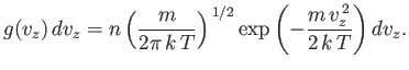 | (vii.212) |
Of course, this expression is properly normalized, so that
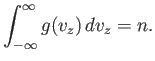 | (7.213) |
Information technology is clear that each component (because there is nothing special about the ![]() -component) of the velocity is distributed with a Gaussian probability distribution (see Department ii.9), centered on a mean value
-component) of the velocity is distributed with a Gaussian probability distribution (see Department ii.9), centered on a mean value
| | (7.214) |
with variance
 | (7.215) |
Equation (7.214) implies that each molecule is just as likely to exist moving in the plus
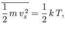 | (7.216) |
in accordance with the equipartition theorem.
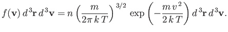
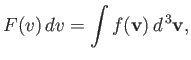
Note that Equation (7.209) can be rewritten
![$\displaystyle \frac{ f({\bf v}) d^{ 3}{\bf v}}{n} =\left[\frac{g(v_x) dv_x... ...\right] \left[\frac{g(v_y) dv_y}{n}\right]\left[\frac{g(v_z) dv_z}{n}\right],$](https://farside.ph.utexas.edu/teaching/sm1/Thermalhtml/img1716.png) | (7.217) |
where
Suppose that we now wish to summate ![]() : that is, the boilerplate number of molecules per unit volume with a speed
: that is, the boilerplate number of molecules per unit volume with a speed ![]() in the range
in the range ![]() to
to ![]() . It is obvious that nosotros can obtain this quantity by summing over all molecules with speeds in this range, irrespective of the direction of their velocities. Thus,
. It is obvious that nosotros can obtain this quantity by summing over all molecules with speeds in this range, irrespective of the direction of their velocities. Thus,
 | (7.218) |
where the integral extends over all velocities satisfying
| | (seven.219) |
This inequality is satisfied by a spherical shell of radius
| | (seven.220) |
which gives
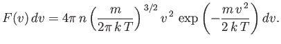 | (7.221) |
This is the famous Maxwell distribution of molecular speeds. Of course, it is properly normalized, so that
 | (7.222) |
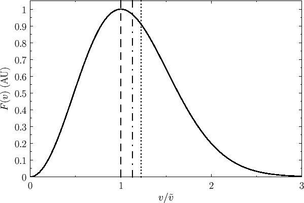
Notation that the Maxwell distribution exhibits a maximum at some non-aught value of
 |
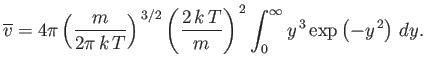
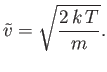
The mean molecular speed is given by
 | (vii.223) |
Thus, we obtain
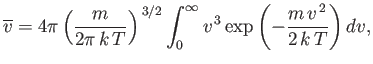 | (7.224) |
or
 | (seven.225) |
Now
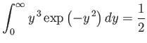 | (7.226) |
(see Do ii), so
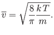 | (vii.227) |
A similar calculation gives
![$\displaystyle v_{\rm rms} = \left[\overline{v^{ 2}}\right]^{ 1/2} = \sqrt{\frac{3 k T}{m}}.$](https://farside.ph.utexas.edu/teaching/sm1/Thermalhtml/img1741.png) | (7.228) |
(See Exercise xiv.) All the same, this event tin also be obtained from the equipartition theorem. Because
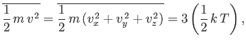 | (7.229) |
then Equation (7.228) follows immediately. It is easily demonstrated that the most likely molecular speed (i.e., the maximum of the Maxwell distribution office) is
 | (7.230) |
The speed of sound in an ideal gas is given by
 | (7.231) |
where
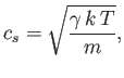 | (7.232) |
considering
Figure 7.7 shows the Maxwell velocity distribution every bit a function of molecular speed in units of the most likely speed. Also shown are the mean speed and the root-mean-square speed.
Next: Effusion Upwards: Applications of Statistical Thermodynamics Previous: Specific Heats of Solids Richard Fitzpatrick 2016-01-25
Source: https://farside.ph.utexas.edu/teaching/sm1/Thermalhtml/node87.html
0 Response to "what is the ratio of mean velocity to maximum velocity?"
Post a Comment